CABB Reduction Example

Data was taken by J Stevens (JBS) and M Voronkov (MV) on the night of 2009-04-01. This experiment is described ​http://svn.atnf.csiro.au/trac/operations/wiki/NFO/Development/CABB/Logs/001,here.

This data is a set of 3-point mosaics on calibrators around 0823-500 and 1934-638. This reduction is to test:

• bandpass stability on calibrators
• mosaic reduction with CABB data
• can we detect polarisation on 1514-241?
• check for decorrelation at offset pointings

Loading the data

For this example I will load only the data from 2009-04-01_1407 onwards as the RA half-power point problem was resolved and the observations include a possibly polarised source 1514-241.

The files we are using are:

4.5G  2009-04-01_1407.C999
4.7G  2009-04-01_1543.C999
2.8G  2009-04-01_1723.C999
1.9G  2009-04-01_1822.C999
3.1G  2009-04-01_1938.C999

for a total of 17G.

First atlod:

atlod% inp
  Task:   atlod
  in       = *.C999
  out      = firstnight_1934.uv
  ifsel    =  
  restfreq =  
  options  = noif
  nfiles   =  
  nscans   =  

We use options=noif since there are actually 4 IFs in each CABB file: IFs 1 & 2 are the 2 GHz 2048 channel wide-bands, while IFs 3 and 4 are the 4096 channel areas that the zoom bands will use. Since the IFs have different numbers of channels, ATLOD will fail if you ask it to map the IFs to the same channel axis. After using options=noif you may select the different IFs using the select=window options.

Let's look at the data using uvplt (this takes quite a while with all the data!):

uvplt% inp
  Task:   uvplt
  vis      = firstnight_1934.uv/
  line     =  
  select   = -auto,window(1),pol(xx,yy)
  stokes   =  
  axis     = time,amp
  xrange   =  
  yrange   =  
  average  =  
  hann     =  
  inc      =  
  options  = nobase
  subtitle =  
  device   = firstnight_firstlook.png/png
  nxy      =  
  size     =  
  log      =  
  comment  =  

This image shows us that something weird happened - we didn't observe on April 2! A quick uvindex shows the problem:

uvindex% inp
  Task:   uvindex
  vis      = firstnight_1934.uv/
  interval =  
  log      =  
  options  =  

09APR01:16:58:33.2 aa1              n  6      2049        0      1  318505
09APR01:16:59:34.0 aa2              n  6      2049        0      1  321097
09APR01:17:00:34.0 aa3              n  6      2049        0      1  323689
09APR02:17:01:27.4 aa3              n  6      2049        0      1  326009
09APR02:17:02:03.2 bb1              n  6      2049        0      1  326225
09APR02:17:03:04.0 bb2              n  6      2049        0      1  328817
09APR02:17:04:04.0 bb3              n  6      2049        0      1  331409
09APR01:17:05:38.2 cc1              n  6      2049        0      1  334001
09APR01:17:06:39.0 cc2              n  6      2049        0      1  336593
09APR01:17:07:39.0 cc3              n  6      2049        0      1  339185

A little quirk has meant that the timestamp is wrong for a few scans. Since the quirk may have also corrupted the data, we take no chances and flag it out with uvflag:

uvflag% inp
  Task:   uvflag
  vis      = firstnight_1934.uv/
  select   = time(09APR02:00:00:00)
  line     =  
  edge     =  
  flagval  = flag
  options  =  
  log      =  

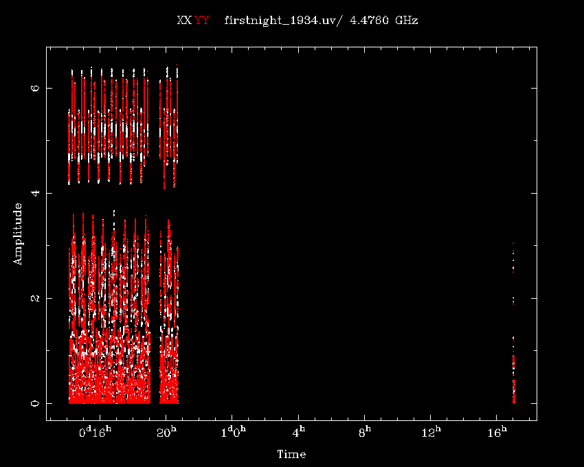
And looking at the data again shows us the following plot.

So we can see that we are observing different sources and that the data looks as one would expect it to. Now let's just look at 1934-638, as we will use it as our primary calibrator.

uvplt% inp
  Task:   uvplt
  vis      = firstnight_1934.uv/
  line     =  
  select   = -auto,window(1),pol(xx,yy),source(aa1)
  stokes   =  
  axis     = time,amp
  xrange   =  
  yrange   =  
  average  =  
  hann     =  
  inc      =  
  options  = nobase
  subtitle =  
  device   = 1/xs
  nxy      =  
  size     =  
  log      =  
  comment  =  

Here we use the source name aa1 for the mosaic pointing on 1934-638 with no offset.

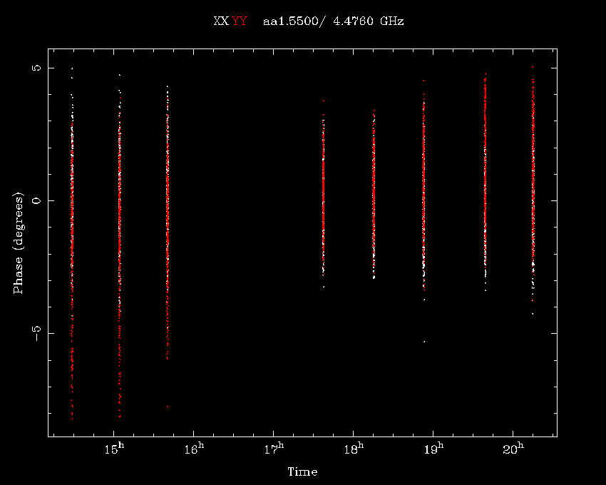
And we can plot phase too:

And the bandpass:

uvspec% inp
  Task:   uvspec
  vis      = firstnight_1934.uv/
  select   = -auto,window(1),pol(xx,yy),source(aa1)
  line     =  
  stokes   =  
  interval = 10
  hann     =  
  offset   =  
  options  = nobase,avall
  axis     = freq,amp
  yrange   =  
  device   = firstnight_1934b_beforecal.png/png
  nxy      = 3,4
  log      =  

We want to calibrate now, but before we do we will need to change the name of the source aa1 to 1934-638, otherwise mfcal won't know to use the 1934 model for the spectral index. This means we have to use uvsplit first:

uvsplit% inp
  Task:   uvsplit
  vis      = firstnight_1934.uv/
  select   =  
  options  =  
  maxwidth =  

Now we use puthd to change the source name:

uvsplit% tget puthd
  Task:   puthd
  in       = aa1.5500/source
  value    = 1934-638
  type     =  

Now we calibrate:

mfcal% inp
  Task:   mfcal
  vis      = aa1.5500
  line     =  
  stokes   =  
  edge     =  
  select   = window(1)
  flux     =  
  refant   =  
  minants  =  
  interval = 0.1
  options  =  
  tol      =  

Here's what the data looks like after calibration pass 1:

First thing we notice is that the edges don't work very well, so we'll flag 50 channels on each edge (100 MHz of total flagging!), and we'll also flag out channels 641 and 1409 which have some RFI. After that we run mfcal again.

Although the calibration doesn't look all that good, we are not getting the whole picture. When we remove antenna 6 (a sensible move since we are in the EW352 configuration), we get: