Reducing CABB Data

An example

This page will walk through the reduction process for the ToO observation CX167, which was observed on 16 Feb 2009 with the interim CABB system. This system had 5 antenna dual pol, 1 IF at 6/3cm, but not all 2048 continuum channels were working.

First, make sure you have the CABB version of MIRIAD, otherwise this will not work!

To do this on kaputar, make sure that /nfs/atapplic/miriad-cabb/linux64/bin is in your path ahead of any other MIRIAD directories. To check that this is so, in a terminal, type which atlod. It should return /nfs/atapplic/miriad-cabb/linux64/bin/atlod.

Then source /nfs/atapplic/miriad-cabb/MIRRC. You should now be using the CABB version of MIRIAD.

To begin with, the reduction is the same as any other pre-CABB dataset, and we start by using ATLOD to read in the data. We have four files for CX167: 2009-02-16_0658.CX167, 2009-02-16_0701.CX167, 2009-02-16_1651.CX167 & 2009-02-16_1824.CX167.

atlod in=*.CX167 out=cx167.uv ifsel=2 options=birdie

Here, we use ifsel=2 because only 1 IF was available with the interim CABB system and it was written as IF 2.

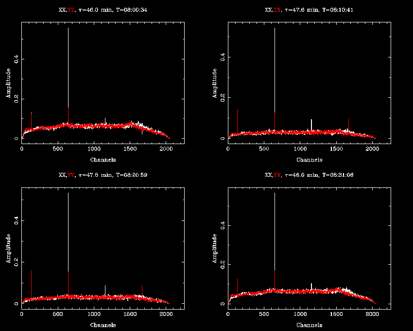
At this point, we can see what the CABB spectrum looks like with uvspec:

uvspec vis=cx167.uv "select=pol(xx,yy)" interval=10 options=nobase,avall axis=chan,amp device=/xs

We want to calibrate the bandpass. Luckily there is some 1934-638 data, so we calibrate our bandpass with that:

mfcal vis=cx167.uv "select=source(1934-638)" interval=0.1

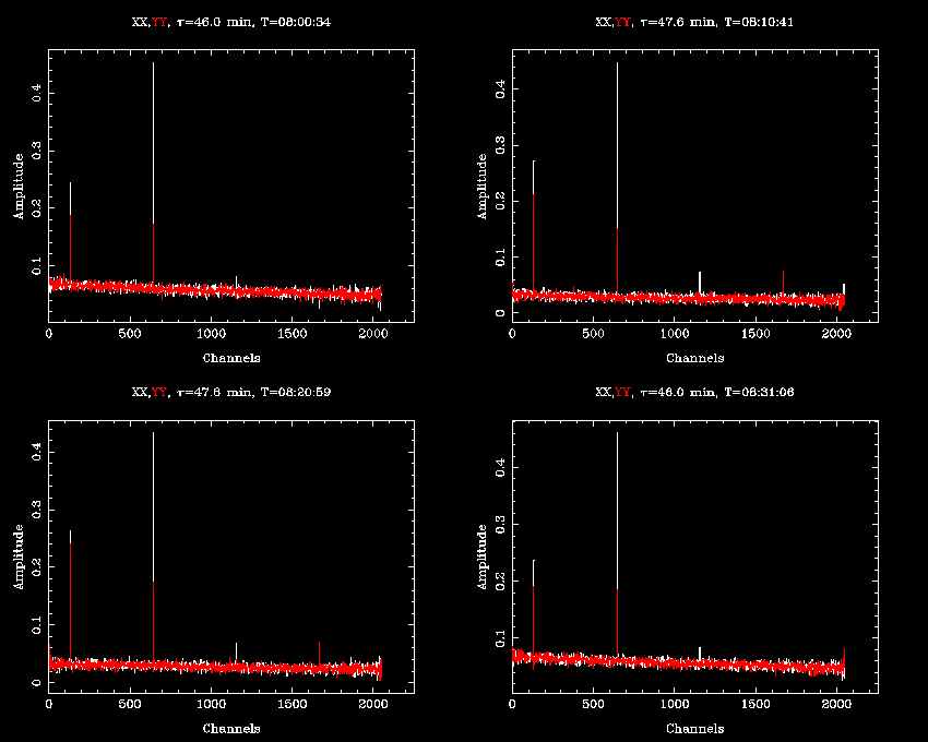
Giving the same uvspec command as before we now get:

There is some obvious narrowband interference present in the data. With CABB's polyphase filter design, the channels are designed to be very sharp-edged, so most interference will be present only in one channel, even if it is very strong. This should allow us to very effectively excise this RFI with an automated routine.

One option is to use Pieflag, Enno Middleberg's automatic flagging script. It works by looking at each channel in turn through time, and finding outliers in comparison to a channel that is known not to have RFI. This works quite well for continuum datasets from the old correlator, since there are fewer channels. Pieflag loads the entire dataset into memory, which can be quite a strain on a computer that does not have enough memory for the datasets that CABB will produce.

Another option is to use a script made by Jamie Stevens to look for narrowband RFI (which is attached to this page). This script looks for individual channels that deviate from the median by more than an acceptable amount.

To search the data for narrowband RFI, give the command:

cabb_nb_rfi_extractor.pl --doit --select-options "-auto,-ant(6)" --interval 10 --flagscript --vis cx167.uv --sigma 5

The script finds that there is interference in channels 5, 133, 645, 1149, 1150, 1157 and 1669. It makes another script which contains the uvflag commands required to flag these channels, which can then be executed.

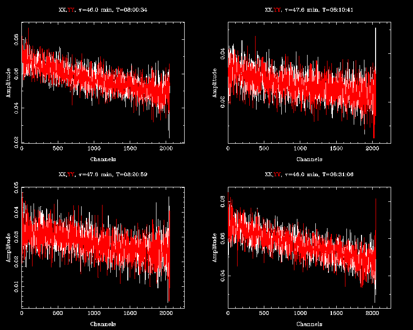
After flagging, the bandpasses look like this:

There seems to be higher noise levels towards the edge of the band, especially at the high channel end, so we use uvflag to clip off 50 channels from each side of the bandpass:

uvflag vis=cx167.uv edge=50 flagval=flag

It should also be noted that the RFI detection script only flags RFI channels that persist throughout most of the intervals that are examined. This behaviour can be changed by telling the script to flag each interval separately (using the --nearby option, or by setting the --persistent flag to be a lower number than the default 30%.

The upshot is that at this point there is still some RFI present, ie. channel 513, during the first observations of 1934-638.

The next step is to recalibrate the dataset again after removing most of the RFI.

mfcal vis=cx167.uv "select=source(1934-638)" interval=0.1

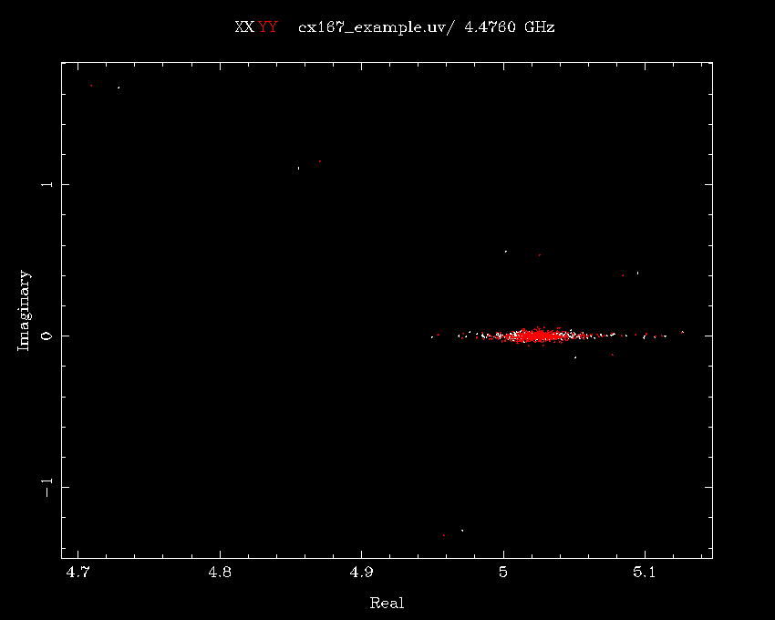
Let's look at the calibration of 1934-638.

uvplt vis=cx167.uv "select=-auto,-ant(6),pol(xx,yy),source(1934-638)" axis=real,imag options=nobase device=/xs

It's not bad, but there are enough outliers to warrant a closer look. A time-phase plot shows the problem:

uvplt vis=cx167.uv "select=-auto,-ant(6),pol(xx,yy),source(1934-638)" axis=time,phase options=nobase device=/xs

The time between 07:09:00 and 07:09:10 has bad phases, so we flag this out:

uvflag vis=cx167.uv "select=time(07:09:00,07:09:10)" flagval=flag

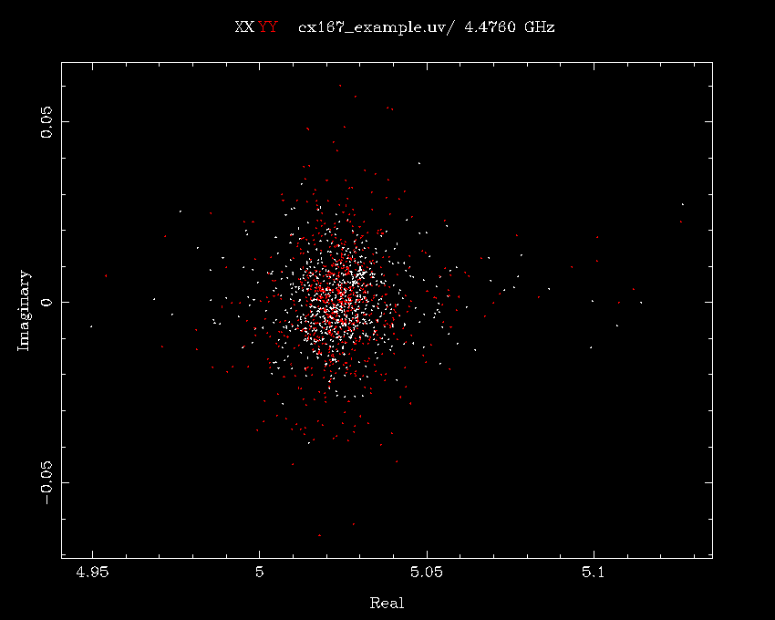
and recalibrate as before. The real,imag plot now looks like this:

Not perfect, but it is good enough for now.

The next step is where CABB reduction really differs from that of the old correlator. We need to determine whether we want to attack the dataset as a whole, working with all 2 GHz of bandwidth simultaneously, or do we want to "divide and conquer" by splitting the band into chunks similar to those output by the old correlator and that we know will work fine with MIRIAD?

In this example we will look at how to proceed in both directions, but we will go through the "divide and conquer" (DAC) procedure first.

To begin the DAC procedure, we use the new CABB uvsplit to split the visibility file, not only based on source, but into fixed bandwidth chunks. Since we know that 128 MHz bandwidth works in MIRIAD, we choose this for uvsplit:

uvsplit vis=cx167.uv select=-auto,-ant(6) maxwidth=0.128

This produces visibility sets for 1934-638, 0515-674 and rnovalmc, at centre frequencies (in MHz) of 4540, 4668, 4796, 4924, 5052, 5180, 5308, 5436, 5564, 5692, 5820, 5948, 6076, 6204, 6332 and 6460; a total of 16 bands (16 x 128 MHz = 2048 MHz, the actual bandwidth of CABB).

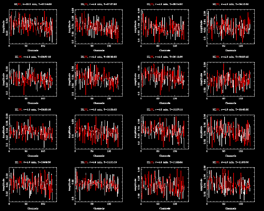
Let's look at the bandpass for one of the bandwidth chunks of the secondary calibrator 0515-674:

uvspec vis=0515-674.5436 "select=pol(xx,yy)" interval=10 options=nobase,avall axis=chan,amp device=/xs nxy=4,4

The bandpasses look pretty good. Note that although we are using 128 MHz bandwidth, the same as was possible with the old correlator, we have 128 channels across the bandwidth, instead of 32 which was usually found with the old correlator.

We should now calibrate the secondary with mfcal, in the same way that it would have been done with old data. However, to do this requires a lot of repetition. This repetition can be handled quickly using the dac_repeat.pl script that is attached to this webpage. It works for any MIRIAD task that you want to run in the same way for multiple visibility sets. For example, to run mfcal on each secondary set, give the following command:

dac_repeat.pl --task mfcal --repeat vis --repeat-freq 0515-674 interval=0.1

The script will find all the frequencies that 0515-674 was observed at and repeat the command

mfcal vis=0515-674.???? interval=0.1

for each set. It can also be used to vary multiple inputs, so we can automatically generate postscript plots for each set, letting the script change the name of the file each time:

dac_repeat.pl --task uvplt --repeat vis --repeat-freq 0515-674 --repeat device --repeat-freq 0515-674_%f.ps/cps axis=real,imag options=nobase

The script will repeat the command

uvplt vis=0515-674.???? device=0515-674_????.ps/cps axis=real,imag options=nobase

because the %f format modifier makes the script substitute the available frequencies.

Going through the plots, it seems that all bands look pretty good except for at 5308 MHz (centre). Looking at its phase shows us that the phase between 12:41:40 and 12:42:00 is bad. It is probably a good idea to flag out that time for all files:

dac_repeat.pl --task uvflag --repeat vis --repeat-freq 0515-674 flagval=flag "select=time(12:41:40,12:42:00)"

After re-running mfcal on each set, we now can see that the data quality on the secondary is good enough to continue.

Now we must use gpboot to correct the gain tables using the 1934-638 data:

dac_repeat.pl --task gpboot --repeat vis --repeat-freq 0515-674 --repeat cal --repeat-freq 1934-638

Now we're ready to copy the calibration tables across to the source files:

dac_repeat.pl --task gpcopy --repeat vis --repeat-freq 0515-647 --repeat out --repeat-freq rnovalmc

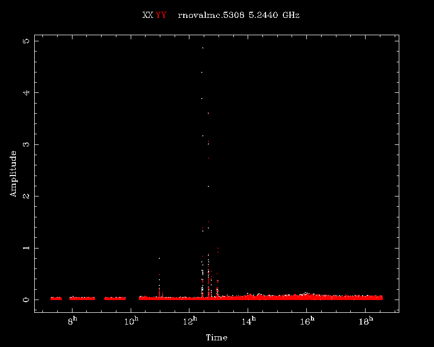
Before we make an image, we can very quickly check for strong interference in the source data:

dac_repeat.pl --task uvplt --repeat vis --repeat-freq rnovalmc --repeat device --repeat rnovalmc_%f.ps/cps axis=time,amp options=nobase "select=-auto,-ant(6),pol(xx,yy)"

Again we find that in the band centred on 5308 MHz there is some strong interference:

The interference is present at the time ranges:

10:58:30 -> 10:58:50

11:05:00 -> 11:05:20

12:25:30 -> 12:25:40

12:26:30 -> 12:26:50

12:27:20 -> 12:27:40

12:38:50 -> 12:40:30

12:44:30 -> 12:44:50

12:55:45 -> 12:59:15

It is probably just narrowband RFI since it is not visible in any other band, so we flag these times in this band only.

Now we are ready to image the source. In the DAC method, there are three ways to make images of the source without recombining the UV data first. We will attempt all three methods:

1. invert using the MFS option as normal, then clean and restor
2. invert using both the MFS option and the SDB option, then use mfclean and restor
3. invert making a cube of all channels, then clean, restor and then make a moment map

The first way is the way most familiar to MIRIAD users doing continuum reduction. We can make images of all the individual datasets in the following way:

dac_repeat.pl --task invert --repeat vis --repeat-freq rnovalmc --repeat map --repeat-freq rnovalmc_%f.map --repeat beam --repeat-freq rnovalmc_%f.beam "select=-auto,-ant(6)" stokes=ii options=double,mfs slop=1

This makes 16 each of the .map and .beam files. Let's get an idea of the RMS noise of each of the maps using imstat. Using kvis we can identify a region (xmin,ymin,xmax,ymax)=(39,0,65,22) that contains no emission. Using dac_repeat.pl we can run imstat on each set:

./dac_repeat.pl --task imstat --repeat in --repeat-freq rnovalmc_%f.map "region=boxes(39,0,65,22)" axes=ra,dec

From this we find that the RMS noise values are:

f (MHz)	RMS (uJy/beam)
4540	246
4668	214
4796	294
4924	385
5052	340
5180	426
5308	351
5436	343
5564	561
5692	386
5820	355
5948	336
6076	444
6204	340
6332	203
6460	179

This gives us an average RMS of 338 uJy. We can use this value when cleaning; we tell clean to stop when it reaches 3 times this value (or 1.014 mJy/beam):

./dac_repeat.pl --task clean --repeat map --repeat-freq rnovalmc_%f.map --repeat beam --repeat-freq rnovalmc_%f.beam --repeat out --repeat-freq rnovalmc_%f.clean cutoff=0.001014

And finally we do restor:

./dac_repeat.pl --task restor --repeat model --repeat-freq rnovalmc_%f.clean --repeat beam --repeat-freq rnovalmc_%f.beam --repeat map --repeat-freq rnovalmc_%f.map --repeat out --repeat-freq rnovalmc_%f.restor

We can see graphic evidence of why we are using the DAC method from the output of our restor commands:

executing [restor model=rnovalmc_4540.clean beam=rnovalmc_4540.beam map=rnovalmc_4540.map out=rnovalmc_4540.restor]
Restor: version 1.3 07- Feb-2002
Using gaussian beam fwhm of   26.672 by   22.525 arcsec.
Position angle:   51.5 degrees.
executing [restor model=rnovalmc_4668.clean beam=rnovalmc_4668.beam map=rnovalmc_4668.map out=rnovalmc_4668.restor]
Restor: version 1.3 07- Feb-2002
Using gaussian beam fwhm of   25.265 by   21.494 arcsec.
Position angle:   52.4 degrees.
executing [restor model=rnovalmc_4796.clean beam=rnovalmc_4796.beam map=rnovalmc_4796.map out=rnovalmc_4796.restor]
Restor: version 1.3 07- Feb-2002
Using gaussian beam fwhm of   24.635 by   20.907 arcsec.
Position angle:   53.5 degrees.
executing [restor model=rnovalmc_4924.clean beam=rnovalmc_4924.beam map=rnovalmc_4924.map out=rnovalmc_4924.restor]
Restor: version 1.3 07- Feb-2002
Using gaussian beam fwhm of   23.992 by   20.378 arcsec.
Position angle:   52.8 degrees.
executing [restor model=rnovalmc_5052.clean beam=rnovalmc_5052.beam map=rnovalmc_5052.map out=rnovalmc_5052.restor]
Restor: version 1.3 07- Feb-2002
Using gaussian beam fwhm of   23.463 by   19.901 arcsec.
Position angle:   52.2 degrees.
executing [restor model=rnovalmc_5180.clean beam=rnovalmc_5180.beam map=rnovalmc_5180.map out=rnovalmc_5180.restor]
Restor: version 1.3 07- Feb-2002
Using gaussian beam fwhm of   22.910 by   19.483 arcsec.
Position angle:   53.7 degrees.
executing [restor model=rnovalmc_5308.clean beam=rnovalmc_5308.beam map=rnovalmc_5308.map out=rnovalmc_5308.restor]
Restor: version 1.3 07- Feb-2002
Using gaussian beam fwhm of   22.394 by   19.020 arcsec.
Position angle:   54.8 degrees.
executing [restor model=rnovalmc_5436.clean beam=rnovalmc_5436.beam map=rnovalmc_5436.map out=rnovalmc_5436.restor]
Restor: version 1.3 07- Feb-2002
Using gaussian beam fwhm of   21.931 by   18.553 arcsec.
Position angle:   55.4 degrees.
executing [restor model=rnovalmc_5564.clean beam=rnovalmc_5564.beam map=rnovalmc_5564.map out=rnovalmc_5564.restor]
Restor: version 1.3 07- Feb-2002
Using gaussian beam fwhm of   21.531 by   18.208 arcsec.
Position angle:   55.1 degrees.
executing [restor model=rnovalmc_5692.clean beam=rnovalmc_5692.beam map=rnovalmc_5692.map out=rnovalmc_5692.restor]
Restor: version 1.3 07- Feb-2002
Using gaussian beam fwhm of   21.018 by   17.827 arcsec.
Position angle:   53.7 degrees.
executing [restor model=rnovalmc_5820.clean beam=rnovalmc_5820.beam map=rnovalmc_5820.map out=rnovalmc_5820.restor]
Restor: version 1.3 07- Feb-2002
Using gaussian beam fwhm of   20.568 by   17.428 arcsec.
Position angle:   53.0 degrees.
executing [restor model=rnovalmc_5948.clean beam=rnovalmc_5948.beam map=rnovalmc_5948.map out=rnovalmc_5948.restor]
Restor: version 1.3 07- Feb-2002
Using gaussian beam fwhm of   20.152 by   17.082 arcsec.
Position angle:   52.6 degrees.
executing [restor model=rnovalmc_6076.clean beam=rnovalmc_6076.beam map=rnovalmc_6076.map out=rnovalmc_6076.restor]
Restor: version 1.3 07- Feb-2002
Using gaussian beam fwhm of   19.800 by   16.781 arcsec.
Position angle:   53.0 degrees.
executing [restor model=rnovalmc_6204.clean beam=rnovalmc_6204.beam map=rnovalmc_6204.map out=rnovalmc_6204.restor]
Restor: version 1.3 07- Feb-2002
Using gaussian beam fwhm of   19.379 by   16.469 arcsec.
Position angle:   53.6 degrees.
executing [restor model=rnovalmc_6332.clean beam=rnovalmc_6332.beam map=rnovalmc_6332.map out=rnovalmc_6332.restor]
Restor: version 1.3 07- Feb-2002
Using gaussian beam fwhm of   19.053 by   16.110 arcsec.
Position angle:   52.0 degrees.
executing [restor model=rnovalmc_6460.clean beam=rnovalmc_6460.beam map=rnovalmc_6460.map out=rnovalmc_6460.restor]
Restor: version 1.3 07- Feb-2002
Using gaussian beam fwhm of   19.330 by   16.151 arcsec.
Position angle:   54.0 degrees.

The beam FWHM changes by around 40% from the bottom of the band to the top.

Let's look at some of the restor'd maps now.

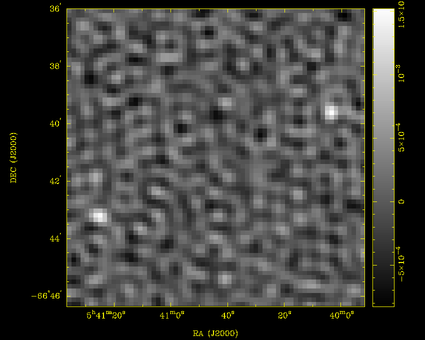
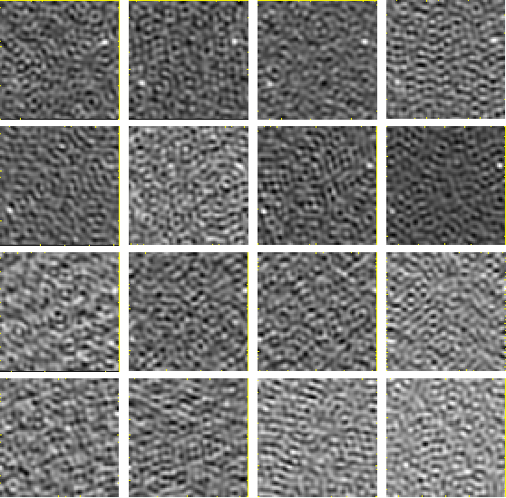
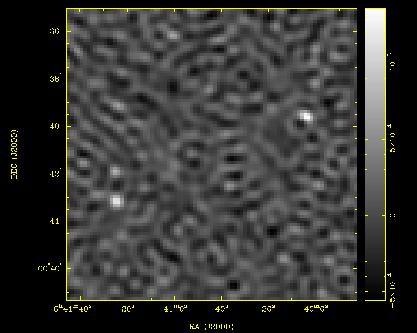
Above is an image of the field with central frequency 4668 MHz. The ToO target is at RA = 05h40m44.2s Dec = -66d40m11.6. So it seems that we have not detected the target, but there are two other sources apparent in the image. Using NED we can identify these sources as SUMSS J054003-663939 (RA = 05h40m03.7s Dec = -66d39m40s, top right source) and SUMSS J054125-664307 (RA = 05h41m25.2s Dec = -66d43m07s, bottom left source). Let's look at all the images together in the image below.

In this image, the central frequency is increasing in each successive plot to the right and down. We can see here another effect of the increasing central frequency. The two sources are seen to "move" towards the edge of the field in successive images, and this is because the primary beam of the antenna gets smaller with increasing frequency.

So we can compare these results with the other methods of imaging, we make some rough measurements of flux of each source. According to NED, SUMSS J054003-663939 has a flux of 1.27 mJy at 843 MHz, and SUMSS J054125-664307 has a flux of 0.94 mJy at 843 MHz.

We get our fluxes using kvis, by taking the sum of the flux in 9 pixels (3x3) centred on the brightest pixel of each source. This should be approximately 1 beam, so we can normalise the flux in the images. The table below shows how the flux of the sources varies with frequency. Note that at a frequency of 5692 MHz the sources are right on the edge of the image, so no measurements are done at frequencies higher than this.

Central Freq (MHz)	J054003-663939 (mJy)	J054125-664307 (mJy)
4540	8.8 +- 2.2	n/a
4668	9.0 +- 1.9	9.0 +- 1.9
4796	10.2 +- 2.6	8.7 +- 2.6
4924	9.5 +- 3.4	7.6 +- 3.4
5052	n/a	12.0 +- 3.0
5180	9.2 +- 3.6	n/a
5308	10.9 +- 3.0	11.1 +- 3.0
5436	14.5 +- 2.8	10.4 +- 2.8
5692	10.7 +- 3.3	8.5 +- 3.3

The sources don't appear to vary in flux much with frequency, at least within the errors of measurement. That would suggest that using mfclean instead of clean might not produce a different result. Let's see!

To begin with we need to redo the invert stage. At this stage we need to use the SDB option as well as the MFS option, The SDB option adds another plane to the beam dataset which represents the change in beam with frequency. We also need to make the beam 3 times the size of the area being cleaned, instead of using options=double which simply doubles the beam size compared to the image. To do this we need to make the image 3 times bigger than the primary beam and then specify the normal imaging region during mfclean. Since the parameters we need to do this will be different for each central frequency, we will control dac_repeat.pl with a parameter file.

We first need to calculate the primary beam size of the antenna for each central frequency, which is simply

1.22 * (c/f) / D

where c is the speed of light, f is the central frequency and D is the diameter of the telescope, in this case 22m. Using this information, and the beam sizes that were computed during the restor operations above, we can determine the image sizes (in pixels) that we need to image 3 times the primary beam size. All this information is in the table below.

Centre Freq (MHz)	Primary Beam (arcmin)	Synthesised beam (arcsec)	Image size (pixels)
4540	12.589	26.672 x 22.525	255 x 302
4668	12.243	25.265 x 21.494	262 x 308
4796	11.917	24.635 x 20.907	261 x 308
4924	11.607	23.992 x 20.378	261 x 308
5052	11.313	23.463 x 19.901	260 x 307
5180	11.033	22.910 x 19.483	260 x 306
5308	10.767	22.394 x 19.020	260 x 306
5436	10.514	21.931 x 18.553	259 x 306
5564	10.272	21.531 x 18.208	258 x 305
5692	10.041	21.018 x 17.827	258 x 304
5820	9.820	20.568 x 17.428	258 x 304
5948	9.609	20.152 x 17.082	257 x 304
6076	9.406	19.800 x 16.781	257 x 303
6204	9.212	19.379 x 16.469	257 x 302
6332	9.026	19.053 x 16.110	256 x 303
6460	8.847	19.330 x 16.151	247 x 296

So we make a file called dac_invert_args.txt that looks like this:

4540 cell=8.891,7.508 imsize=255,302
4668 cell=8.422,7.165 imsize=262,308
4796 cell=8.212,6.969 imsize=261,308
4924 cell=7.997,6.793 imsize=261,308
5052 cell=7.821,6.634 imsize=260,307
5180 cell=7.637,6.494 imsize=260,306
5308 cell=7.465,6.340 imsize=260,306
5436 cell=7.310,6.184 imsize=259,306
5564 cell=7.177,6.069 imsize=258,305
5692 cell=7.006,5.942 imsize=258,304
5820 cell=6.856,5.809 imsize=258,304
5948 cell=6.717,5.694 imsize=257,304
6076 cell=6.600,5.594 imsize=257,303
6204 cell=6.460,5.490 imsize=257,302
6332 cell=6.351,5.370 imsize=256,303
6460 cell=6.443,5.384 imsize=247,296

And we run invert using dac_repeat.pl like this:

dac_repeat.pl --task invert --repeat vis --repeat-freq rnovalmc --repeat map --repeat-freq rnovalmc_m2_%f.map --repeat beam --repeat-freq rnovalmc_m2_%f.beam "select=-auto,-ant(6)" stokes=ii options=mfs,sdb slop=1 --args-file dac_invert_args.txt

This makes the triple-sized maps and beams, and now we have to specify the normal sized map while using mfclean. We make the file dac_mfclean_args.txt that looks like this:

4540 region=relcenter,boxes(-42,-50,42,50)
4668 region=relcenter,boxes(-43,-51,43,51)
4796 region=relcenter,boxes(-43,-51,43,51)
4924 region=relcenter,boxes(-43,-51,43,51)
5052 region=relcenter,boxes(-43,-51,43,51)
5180 region=relcenter,boxes(-43,-51,43,51)
5308 region=relcenter,boxes(-43,-51,43,51)
5436 region=relcenter,boxes(-43,-51,43,51)
5564 region=relcenter,boxes(-43,-50,43,50)
5692 region=relcenter,boxes(-43,-50,43,50)
5820 region=relcenter,boxes(-43,-50,43,50)
5948 region=relcenter,boxes(-42,-50,42,50)
6076 region=relcenter,boxes(-42,-50,42,50)
6204 region=relcenter,boxes(-42,-50,42,50)
6332 region=relcenter,boxes(-42,-50,42,50)
6460 region=relcenter,boxes(-41,-44,41,44)

This is handy since mfclean also requires that the "region being cleaned should be reasonably centred in the map, and should have an appreciable guard band around it to the map edge (of size comparable to the width of the region being cleaned)".

We run mfclean using dac_repeat.pl like this:

dac_repeat.pl --task mfclean --repeat map --repeat-freq rnovalmc_m2_%f.map --repeat beam --repeat-freq rnovalmc_m2_%f.beam --repeat out --repeat-freq rnovalmc_m2_%f.clean --args-file dac_mfclean_args.txt

We can still use restor with MFS datasets, but it will create a triple-sized image, although of course only the central region will be cleaned.

dac_repeat.pl --task restor --repeat model --repeat-freq rnovalmc_m2_%f.clean --repeat beam --repeat-freq rnovalmc_m2_%f.beam --repeat map --repeat-freq rnovalmc_m2_%f.map --repeat out --repeat-freq rnovalmc_m2_%f.restor

If you only want to see the primary beam in your restor'd images, then you can use imframe using the same dac_mfclean_args.txt:

dac_repeat.pl --task imframe --repeat in --repeat-freq rnovalmc_m2_%f.restor --repeat out --repeat-freq rnovalmc_m2_small_%f.restor --args-file dac_mfclean_args.txt